Acme Analytics Regional Sales Analysis

Dashboards

#

Project Summary

#

This project dives into Acme Co.’s 2014–2018 USA sales dataset through:

• Data Profiling & Cleaning: Verified schema, handled missing budgets, and corrected data types.
• Univariate & Bivariate Analysis: Explored distributions (revenue, margin, unit price), product/channel/region breakdowns, and customer segments.
• Trend & Seasonality: Charted monthly and yearly sales patterns, highlighting recurring surges and dips.
• Outlier Detection: Identified extreme transactions at both ends of the revenue and unit-price spectra.
• Correlation & Segmentation: Assessed relationships between key metrics and clustered customers by revenue vs. profit margin.

Problem Statement

#

Analyze Acme Co.’s 2014–2018 sales data to identify key revenue and profit drivers across products, channels, and regions; uncover seasonal trends and outliers; and align performance against budgets. Use these insights to optimize pricing, promotions, and market expansion for sustainable growth and reduced concentration risk.

• Business Questions
  • Inconsistent revenue and profit performance across U.S. regions
  • Lack of visibility into seasonal swings, top SKUs and channel profitability

Objectives

#

Deliver actionable insights from Acme Co.’s 2014–2018 sales data to:

• Identify top-performing products, channels, and regions driving revenue and profit
• Uncover seasonal trends and anomalies for optimized planning
• Spot pricing and margin risks from outlier transactions
• Inform pricing, promotion, and market-expansion strategies

These findings will guide the design of a Power BI dashboard to support strategic decision-making and sustainable growth.

Entity Relationship Diagram

#

erDiagram
    SALES_ORDERS }o--|| CUSTOMERS : places
    SALES_ORDERS }o--|| PRODUCTS : includes
    SALES_ORDERS }o--|| REGIONS : delivers_to
    REGIONS }o--o{ STATE_REGIONS : part_of
    PRODUCTS ||--o{ BUDGETS_2017 : has

    CUSTOMERS {
        int Customer_Index
        string Customer_Names
    }

    PRODUCTS {
        int Index
        string Product_Name
    }

    REGIONS {
        int id
        string name
        string state_code
    }

    SALES_ORDERS {
        string OrderNumber
        date OrderDate
        int Customer_Name_Index
        int Product_Description_Index
        int Delivery_Region_Index
        int Order_Quantity
        float Unit_Price
        float Line_Total
    }

    STATE_REGIONS {
        string State_Code
        string State
        string Region
    }

    BUDGETS_2017 {
        string Product_Name
        float Budget
    }

Project Workflow

#

• Define Busines Objective: Understand the core problem and expected business outcomes.
• Collect & Consolidate Data: Gather multi-source sales data and understand schema.
• Data Loading & Initial Exploration: Load into Colab/Jupyter Notebook for initial profiling and data understanding using Python.
• Pre-processing & Cleaning: Handle nulls, join tables, format dates and normalize columns.
• Exploratory Data Analysis (EDA): Visualize trends, compare performance, and extract key insights.
• Dashboarding & Recommendations: Build Power BI dashboard and present strategic findings.

Exploratory Data Analysis

#

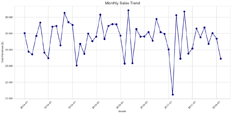
1. Monthly Sales Trend over Time

#

• Goal: Track revenue trends over time to detect seasonality or sales spikes
• Chart: Line chart
• EDA Type: Temporal (time series)
• Structure: Line with markers to highlight monthly revenue points clearly

  

Insights

#

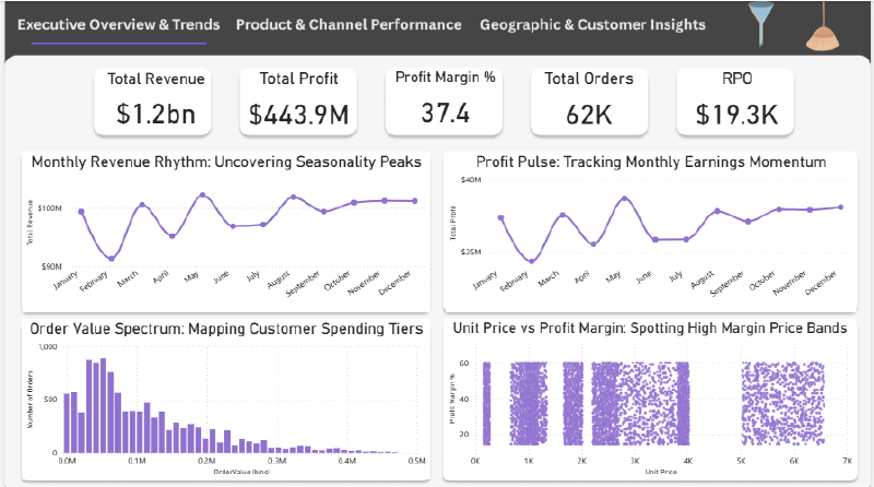
• Sales consistently cycle between 24M and 26M, with clear peaks in late spring to early summer (May–June) and troughs each January.
• The overall trend remains stable year over year, reflecting a reliable seasonal demand pattern.
• However, the sharp revenue drop in early 2017 stands out as an outlier, warranting closer investigation into potential causes such as market disruptions or mistimed promotions.

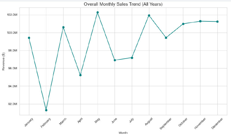
2. Monthly Sales Trend (all years combined)

#

• Goal: Highlight overall seasonality patterns by aggregating sales across all years for each calendar month
• Chart: Line chart
• EDA Type: Temporal (time series)
• Structure: Line with markers, months ordered January to December based on month number

  

Insights

#

• Across all years, January begins strong with roughly 99M, followed by a steep decline through April’s slowpoint(≈ 95M).
• Sales rebound in May and August (≈ 102M) before settling into a pleateau of 99-101M from September to December.
• This pattern reveals a strong post–New Year surge, a spring dip, and a mid–summer bump each calendar year.

3. Top 10 Products by Revenue (in Millions)

#

• Goal: Identify the highest-grossing products to focus marketing and inventory efforts
• Chart: Horizontal Bar chart
• EDA Type: Univariate
• Structure: Bars sorted descending to show top 10 products with revenue scaled in millions

  

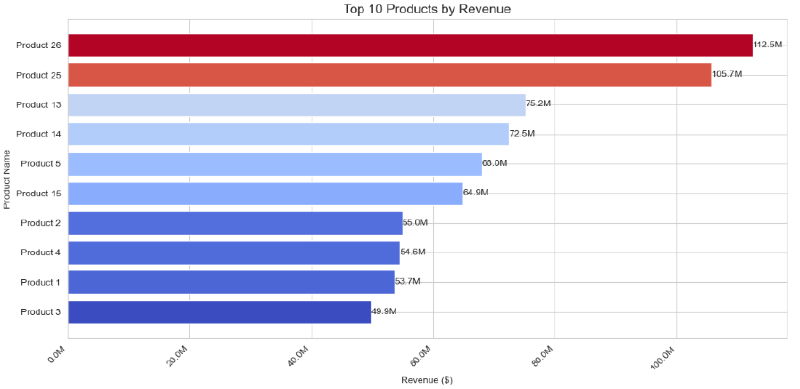
Insights

#

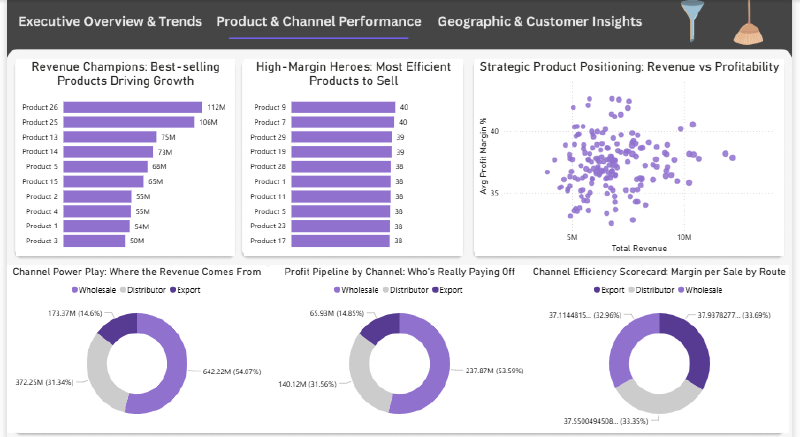
• Products 26 and 25 pull away at 112M and 105M, with a sharp drop to 75M for Product 13 and a tight mid-pack at 64-72M.
• The bottom four cluster at 50-55M, highlighting similar constraints.
• Focus on growth pilots for the mid-tier and efficiency gains for the lower earners to drive significant lifts.

4. Top 10 Products by Average Profit Margin

#

• Goal: Compare average profitability across products to identify high-margin items
• Chart: Horizontal Bar chart
• EDA Type: Univariate
• Structure: Bars sorted descending to show top 10 products with average profit margin values

  

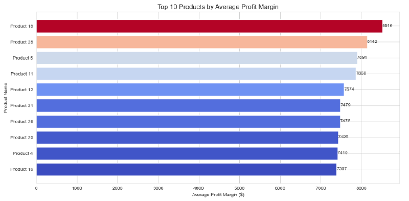
Insights

#

• Products 18 and 28 lead with average profit margins of approximately
• Mid-tier performers like Products 12, 26, and 21 cluster in the
• Focusing on margin optimization strategies from top performers may help elevate overall product profitability.

5. Sales by Channel

#

• Goal: Show distribution of total sales across channels to identify dominant sales routes
• Chart: Pie chart
• EDA Type: Univariate
• Structure: Pie segments with percentage labels, colors for clarity, start angle adjusted

  

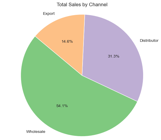
Insights

#

• Wholesale accounts for 54.1% of sales, with distributors at 31.3% and exports at 14.6%, underscoring reliance on domestic bulk channels.
• To diversify revenue and mitigate concentration risk, prioritize expanding export initiatives—through targeted overseas marketing and strategic partner relationships.

6. Average Order Value (AOV) Distribution

#

• Goal: Understand distribution of order values to identify typical spending levels and outliers
• Chart: Histogram
• EDA Type: Univariate
• Structure: Histogram with 50 bins, colored bars with edge highlights to show frequency of order values

  

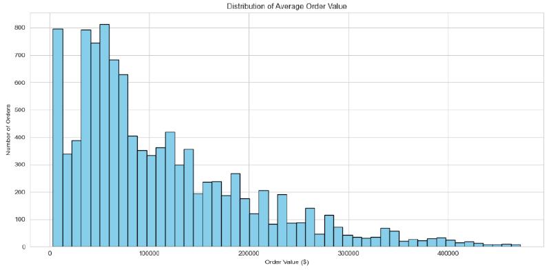
Insights

#

• The order‐value distribution is heavily right‐skewed, with most orders clustering between 20-120K and a pronounced mode around 50-60 K.
• A long tail of high-value transactions extends up toward 400-500K, but these large orders represent only a small share of total volume.

7. Profit Margin % vs. Unit Price

#

• Goal: Examine relationship between unit price and profit margin percentage across orders
• Chart: Scatter plot
• EDA Type: Bivariate
• Structure: Scatter points with transparency to show data density

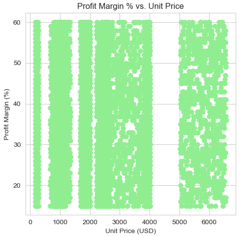
Insights

#

• Profit margins are concentrated between 18% and 60%, with no clear correlation to unit price, which spans from near 0 to over 6,500.
• Dense horizontal bands indicate consistent margin tiers across a wide price spectrum, reflecting uniform pricing strategies.
• Outliers below 18% at both low and high price points may signal cost inefficiencies or pricing issues worth deeper investigation.

8. Unit Price Distribution per Product

#

• Goal: Compare pricing variability across different products to identify price consistency and outliers
• Chart: Boxplot
• EDA Type: Bivariate
• Structure: Boxplot with rotated labels to display unit price spread per product

  

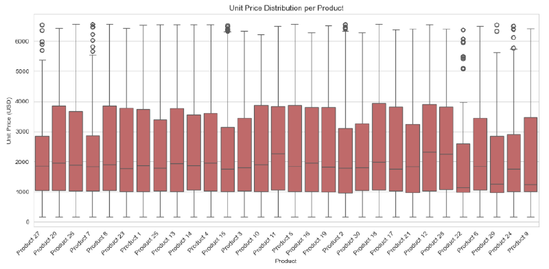
Insights

#

• Products 8, 17, 27, 20, and 28 show high-end revenue spikes - well above their upper whiskers, likely due to bulk orders, special-edition releases, or premium bundles that temporarily inflate earnings.
• In contrast, deep low-end outliers (near 0-100) on Products 20 and 27 suggest promotional giveaways or test SKUs that pull down average prices.
• To ensure accurate margin and pricing assessments, exclude these outlier transactions from average calculations.
• Then assess whether such anomalies warrant formalization as ongoing promotional strategies or should be phased out to stabilize pricing performance.

9. Total Sales by US Region

#

• Goal: Compare total sales across U.S. regions to identify top‑performing markets and areas for targeted growth.
• Chart: Horizontal bar chart
• EDA Type: Univariate comparison
• Structure: Bars sorted ascending (Northeast → West) for clear bottom‑to‑top ranking. X‑axis in millions USD, Y‑axis listing regions

  

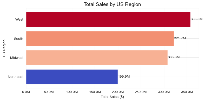
Insights

#

• West dominates with roughly 360M in sales (35% of total), underscoring its market leadership
• South & Midwest each contribute over 320M (32% of total), indicating strong, consistent demand across central regions.
• Northeast trails at about $210 M (~20 %), signaling room for growth and targeted investment.
• Action: Focus on closing the Northeast gap with local promotions and strategic partnerships, while maintaining national playbook success

10. Total Sales by State

#

• Goal: Visualize geographic distribution of sales to identify high- and low-performing states and uncover regional gaps.
• Chart: US choropleth map
• EDA Type: Univariate geospatial
• Structure:
  • States shaded by total sales (in millions USD) using a blue gradient
  • Legend on the right showing sales scale (M USD)
  • Hover tooltips display exact sales for each state
  • Map scoped to USA for clear regional context

    

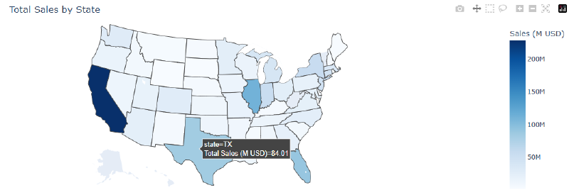
Insights

#

• California leads with 230M followed by Illinois (111M) and Florida (90M).
• Mid‑tier states (e.g. Texas - 55 M) hold steady performance but trail the top three by 40–145M. Lower‑tier states (e.g. New Jersey - 35 M) reveal a gradual drop, indicating uneven market penetration.
• Action: Double down on top states with tailored promotions, and launch targeted growth initiatives in under‑penetrated regions to close the gap

11. Top and Bottom 10 Customers by Revenue

#

• Goal: Identify your highest- and lowest-revenue customers to tailor engagement strategies
• Chart: Side-by-side horizontal bar charts
• EDA Type: Multivariate
• Structure: Left chart shows top 10 customers by revenue (in millions), right chart shows bottom 10 customers by revenue (in millions)

  

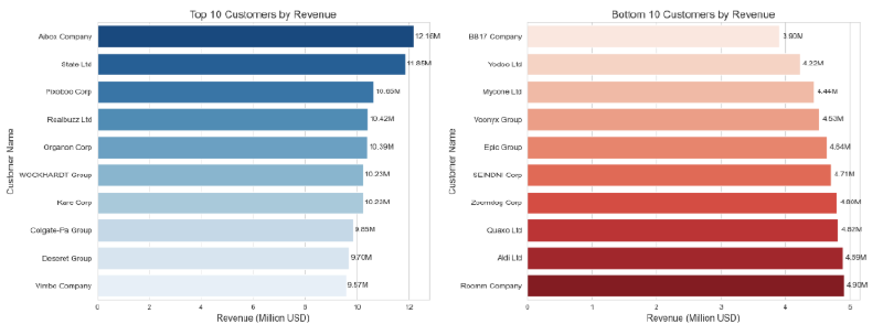
Insights

#

• Aibox Company tops the list with 12.16M followed closely by State Ltd. (11.85M), while the 10th-ranked Vimbo Company still contributes 9.57M demonstrating a tight 10–12 M top tier.
• At the bottom, Roomm Company leads its group with 4.9M, down to BB17 Company at 3.9M - roughly half the top customer’s revenue.
• This steep drop from ~10M to 4–5M highlights high revenue concentration among the top customers.
• Action: prioritize retention and upsell for your top ten, and launch targeted growth campaigns to elevate the lower-revenue cohort.

12. Average Profit Margin by Channel

#

• Goal: Compare average profit margins across sales channels to identify the most and least profitable routes
• Chart: Bar chart
• EDA Type: Bivariate
• Structure: Vertical bars with data labels showing margin percentages, sorted descending by channel

  

Insights

#

• Export leads with a 37.94% average margin, closely followed by Distributor (37.55%) and Wholesale (37.11%).
• The tiny spread (<0.2 %) shows consistently strong profitability across all channels.
• This uniformity implies well-controlled costs and pricing power everywhere.
• To maximize returns, push volume growth in Export while maintaining efficiency in Distributor and Wholesale.

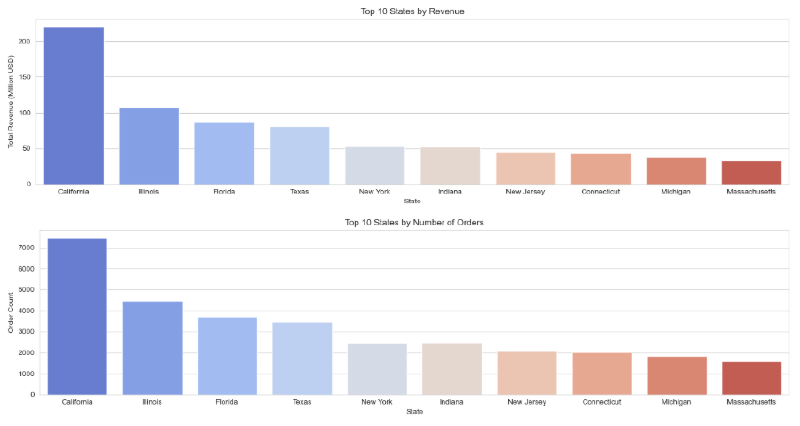
13. Top 10 States by Revenue and Order Count

#

• Goal: Identify highest revenue-generating states and compare their order volumes
• Chart: Two bar charts
• EDA Type: Multivariate
• Structure: First chart shows top 10 states by revenue (in millions), second shows top 10 states by number of orders

  

14. Customer Segmentation: Revenue vs. Profit Margin

#

• Goal: Segment customers by total revenue and average profit margin, highlighting order volume
• Chart: Bubble chart (scatter plot with variable point sizes)
• EDA Type: Multivariate
• Structure: Scatter points sized by number of orders, plotting revenue vs. margin

  

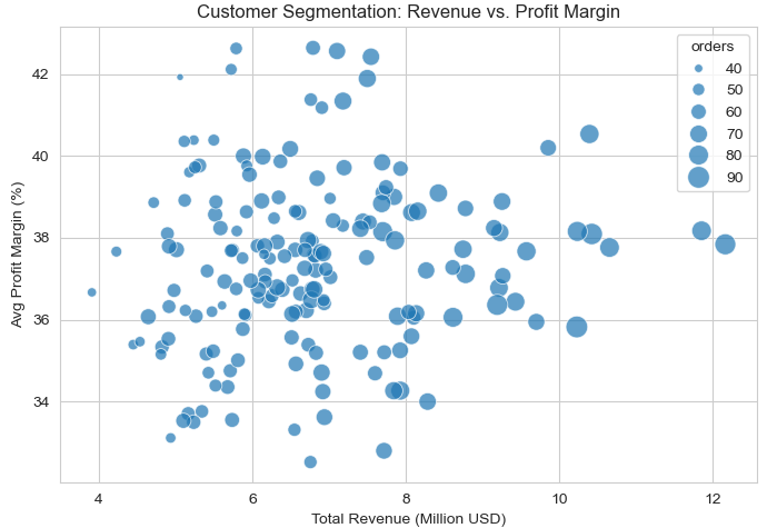
Insights

#

• Customers with >10M in revenue tend to sustain margins between 36–40%, indicating that scale does not significantly erode profitability.
• Most customers cluster within the 6–10M range and show stable margins (~34–40%), suggesting consistent pricing in this tier.
• Customers below 6M display the widest margin variance (~33–43%), pointing to more volatile cost structures or discounts among smaller accounts.
• Bubble size (order count) increases with revenue, but margin levels appear unaffected—reinforcing revenue as the dominant performance driver over order volume.

15. Correlation Heatmap of Numeric Features

#

• Goal: Identify relationships among key numeric variables to uncover potential multicollinearity
• Chart: Correlation heatmap
• EDA Type: Multivariate
• Structure: Annotated heatmap with correlation coefficients for selected numeric columns

  

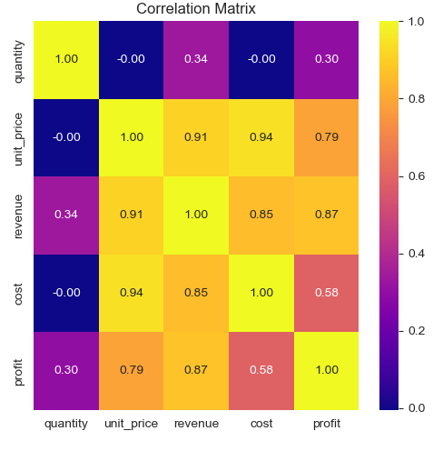
Insights

#

• Profit and revenue are very strongly correlated (0.87), indicating that as sales value increases, profit tends to rise as well.
• Unit price is a key driver: it correlates 0.91 with revenue, 0.79 with profit, and 0.94 with cost—highlighting how pricing decisions ripple through both top‑line and expense figures.
• Cost shows a strong link to revenue (0.85) but a more moderate tie to profit (0.58), underscoring that while higher sales often bring higher expenses, margins can still vary.
• Quantity has virtually no correlation with unit price or cost (≈0.00) and only modest associations with revenue (0.34) and profit (0.30), making volume a secondary factor compared to pricing.

Key Insights

#

• Monthly Revenue Cycle: Revenue stays stable between ≈23M-26.5M across 2014–2017, with no consistent seasonal spikes. Sharpest drop (≈21.2M) occurs in early 2017, indicating a possible one-time disruption.
• Channel Mix: Wholesale: 54%. Distributors: 31%. Exports: 15% — opportunity to scale international presence.
• Top Products (Revenue): Product 26: 112M; Product 25: 106M; Product 13: 75M. Mid-tier: 65–75M; bottom performers: 50–55M.
• Profit Margins: Profit margins range broadly from ≈18% to ≈60%, with no strong correlation to unit price. Dense horizontal bands suggest standardized pricing strategies across tiers.
• Seasonal Volume: No strong monthly pattern, but slight volume uptick appears around May–June. Early 2017 dip (≈21.2M) may require investigation.
• Regional Performance: California leads: ≈230M Revenue & 7500+ orders. Illinois/Florida/Texas: ≈85M–110M & ≈3500–4500 orders. NY/Indiana: ≈54M & 2000+ orders.

Recommendations

#

• Outlier Strategy: Exclude or formalize bulk-order and promotional SKUs when calculating averages.
• Margin Uplift: Apply top-product pricing levers to mid/low tiers; cut costs on underperformers.
• Export Growth: Invest in targeted overseas marketing and distributor partnerships.
• Seasonal Planning: Shift spend toward January trough and May–June peak; investigate the 2017 anomaly.
• Dashboard Prep: Build aggregated tables for time series, channel mix, and product performance for Power BI.